

Deploying STELLA: Field Notes from the Morven Campaign
On a hot summer morning at Morven, the University of Virginia’s research and sustainability site outside Charlottesville, five people stood in a field of tall grass with a handheld spectrometer, measuring the same ground that drones and satellites above were also studying that season.
What they were working toward was trust. STELLA is an open source, build it yourself instrument created by Paul Mirel, lead engineer of NASA’s STELLA Project, designed to be affordable so that anyone with a soldering iron and a few afternoons can build a working instrument for exploration. That accessibility is the whole point, but it also raises an obvious question. Can a low cost, build it yourself sensor be trusted to produce reliable data? Answering that question for real, with numbers behind it, is the work this team went to Morven to begin. Every reading they took in that field is a small piece of evidence toward calibrating STELLA against the lab, and toward showing it can stand alongside the instruments it was built to make more accessible.
A Team Built in the Field
The group came together from very different starting points. Bianca Cilento, who holds a bachelor’s and master’s degree from RIT in environmental science, served as field operations manager. “I helped develop the data plan that we followed, and I instructed everybody on how to use the STELLA,” she said of her role. “And now I’m doing the data analysis of what we collected.” She took on the role as a volunteer.
Joining her was Kelsey Huelsman, a NASA postdoctoral researcher with a background in hyperspectral remote sensing. Kelsey had spent her dissertation flying drone mounted spectrometers over Blandy Experimental Farm to detect invasive plant species. Despite years of experience with similar instruments, this was her first time putting her hands on a STELLA unit. “This was my first time using STELLA, and Bianca taught us well,” she said. “I followed Bianca’s lead in our field work.”
Rounding out the team were three members of the University of Virginia community. Tierney Cantwell, a graduate student working under Manuel Lerdau, helped shape the ecological questions the campaign was built to answer. Emma Ellsworth and Emeline Daley, both undergraduates and fellows in UVA’s Decarbonization Academy, were new to remote sensing when the campaign began.
“I found the instrument, as someone lacking a background in hyperspectral data and measurement, was rather intuitive to use,” Emeline said. “A lot of credit to Bianca for that, and to Paul, and just the general organization of the tool.”
That sentiment came up again and again. What started as a technical field campaign also became a training ground, workforce development in practice rather than in name, with more experienced teammates coaching newcomers through gain settings, integration time, and the small judgment calls that come with working outdoors.



Learning to Read the Land
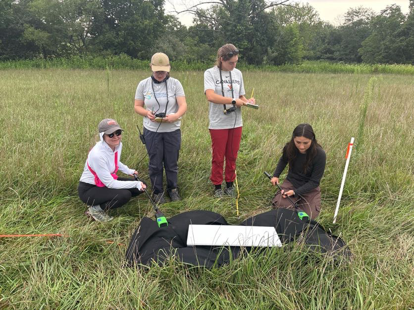
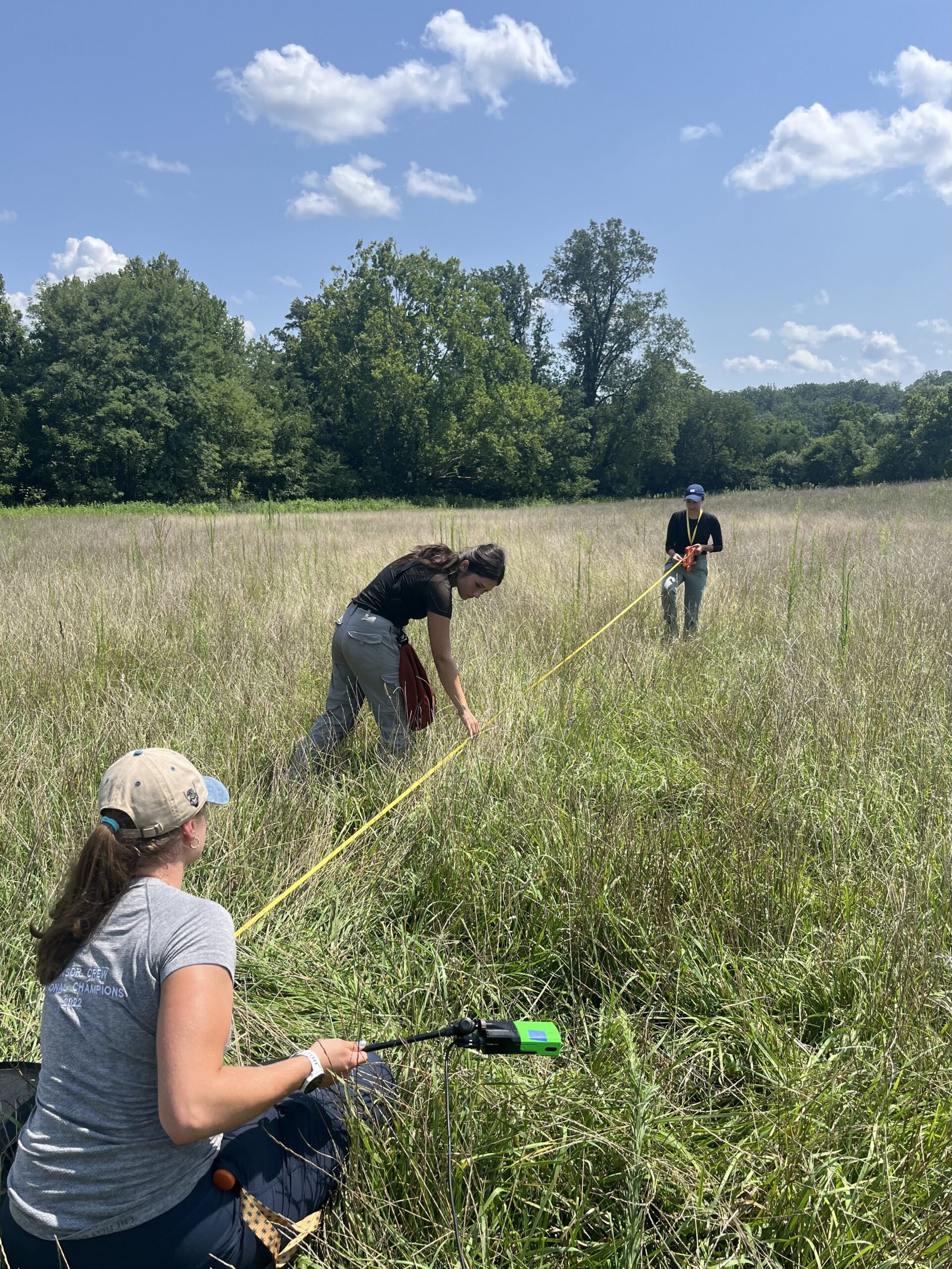
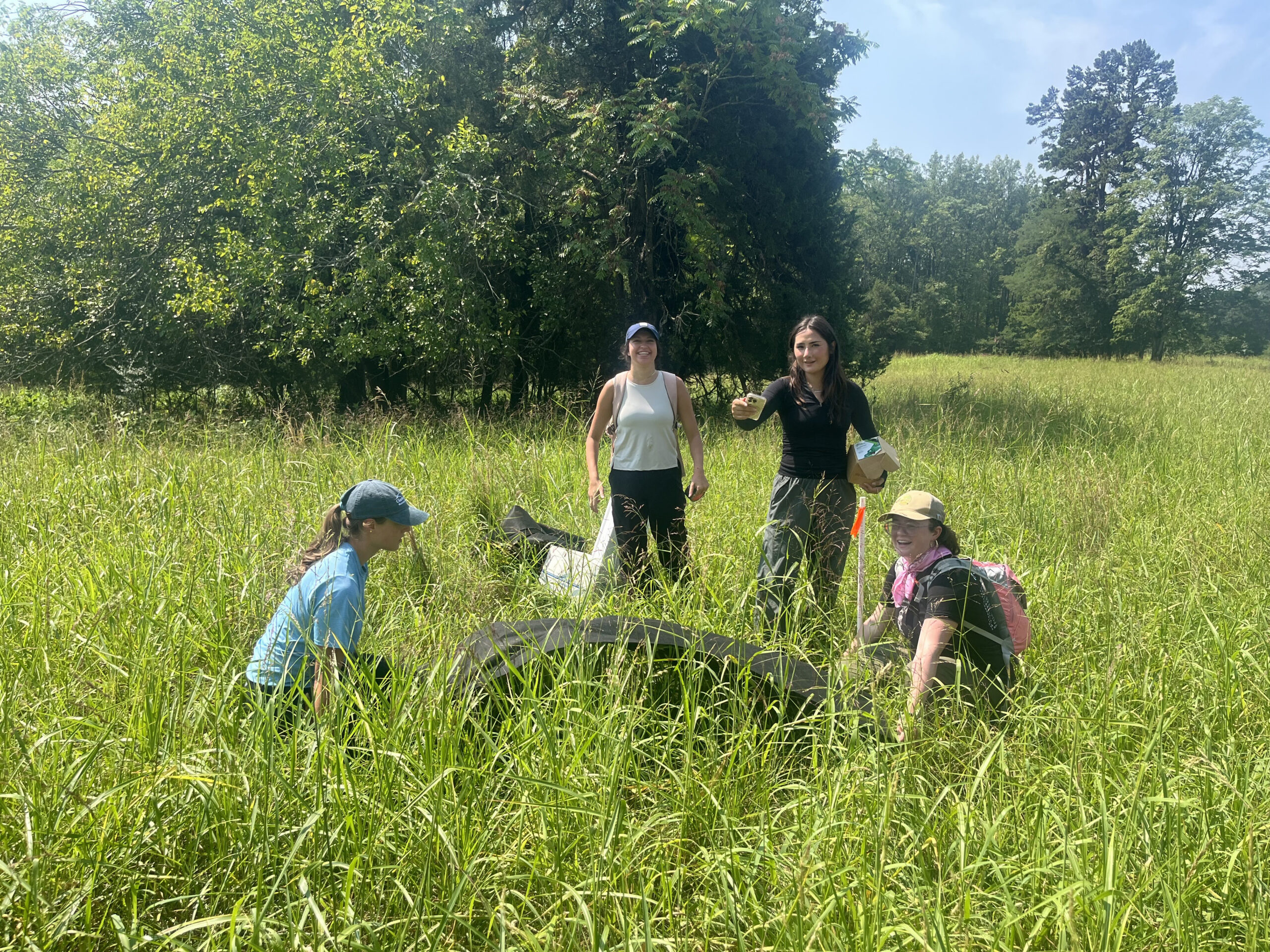
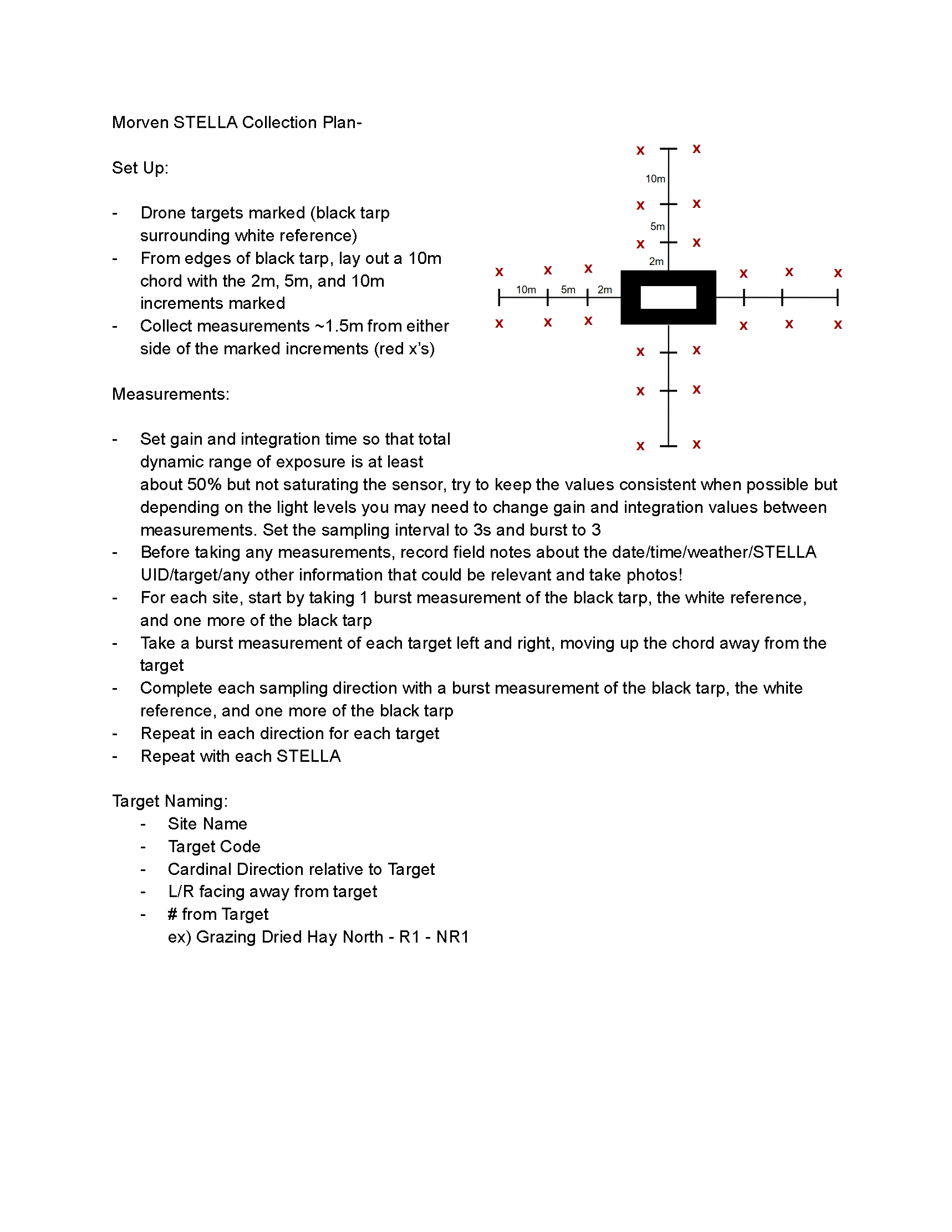
Each day, the team split into two pairs, one person operating STELLA and recording notes, the other holding the sensor steady with an extended tether arm to keep measurements consistent and avoid disturbing the vegetation underfoot. They walked transects out from marked targets, taking calibrated black, white, and black reference readings before capturing the reflectance of the grasses, shrubs, and mixed plant communities around them.
The team also timed its work to align with an airborne survey of the same fields flown under a NASA Advanced Information Systems Technology, or AIST, drone research project, which sent a pair of coordinated drones carrying hyperspectral and thermal cameras over Morven, along with a flyover from G-LiHT, NASA Goddard’s airborne LiDAR, hyperspectral, and thermal imaging platform.
The work was not always easy. Virginia’s weather shifted quickly, and exposure settings had to be adjusted as clouds rolled through. The equipment, still in active development, occasionally overheated in its enclosure. By the later days of the campaign, the team had settled into a steady rhythm. “We really had a rhythm of, you know, we lay out the transect, and we were in teams of two,” Bianca said. “They would walk to their location, one team would go left, one team would go right, take their measurements, and swap. They were a completely well-oiled machine.”
More Than a Field Campaign
Ask the team what stood out most, and the answers point to people as much as data.
For Bianca, who had the most experience with STELLA on the team but had mostly worked with it on her own before this campaign, leading the group was a new experience in itself. “I’ve never really collected STELLA as part of a team before,” she said. “It was so interesting to see the different perspectives, because they all have different backgrounds and different experience levels with remote sensing and ecology and data collection. It was so rewarding to see them play with it themselves and ask their own questions.”
Several team members described wanting to keep working with STELLA beyond this campaign. Tierney, who plans to continue her research at Morven, said simply, “Getting just more measurements there would probably be the first thing that comes to my mind.” Emma, who is starting a senior thesis on Red Oaks, said she was interested in exploring “how STELLA could be used in this project… and how the phenology is changing, or between populations, or how it just generally is responding to the climate here in Virginia.”
None of this would have been possible without Morven itself, the University of Virginia’s living laboratory and sustainability site, which provided the fields, the infrastructure, and the community that made this campaign possible. It also would not have happened without NASA’s STELLA Project, which put remote sensing within reach of students and early career scientists in the first place.
By the end of the campaign, the team had collected consistent measurements across ten sites, data that will help anchor the calibration work needed to define just how accurate STELLA really is. They had also built something harder to measure: a group of scientists, students, and mentors who taught each other and left the field with more than the data they came for.


Citations
Cilento, B., Huelsman, K., Cantwell, T., Ellsworth, E., & Daley, E. (2026, September 13). Deploying STELLA: Field Notes from the Morven Campaign (M. Taylor, Interviewer). https://doi.org/10.17605/OSF.IO/D4ST8
Mirel, P., Taylor, M. P., Barber, W. J., Campbell, P., Cilento, B., Nichols, L. M., and Lerdau, M. (2025). Science and Technology Education for Land/Life Assessment (STELLA): Democratizing Remote Sensing Science With Low-Cost Open-Source Instruments for Research and Education. Perspectives of Earth and Space Scientists. https://doi.org/10.1029/2025CN000284
Interview Transcript
Interviewer: Mike Taylor (NASA GSFC, STELLA Team Lead) Guests: Bianca Cilento, Kelsey Huelsman, Tierney Cantwell, Emma Ellsworth, and Emeline Daley
00:00:04:03 – 00:00:16:09
Hello. My name is Mike Taylor, and I will be the host. I am currently the Stella Project team lead, and I am talking with these awesome folks who went out into the field with some Stellas and Morven, Virginia.
00:00:16:10 – 00:00:18:03
Thank you very much for joining me.
00:00:18:05 – 00:00:25:13
for each of you starting with Bianca, please introduce yourselves, share your academic background and explain what role you played in the field.
00:00:25:14 – 00:00:46:03
Hi, I’m Bianca Cilento. I have my bachelor’s and master’s from RIT in environmental science, and I was the field operations manager of the Stella project at Morven. So I helped develop the data plan that we followed, and I instructed everybody on how to use the Stella. And now I’m doing the data analysis of what we collected.
00:00:46:05 – 00:00:47:00
00:00:47:01 – 00:01:16:06
So I am a postdoctoral researcher at NASA actually, but have never used Stella before. So this was my first time using Estella, and Bianca taught us well. My background is in hyperspectral remote sensing. I used a headwall spectrometer on a drone for my dissertation work, where I was doing flights to try to detect invasive plant species at Blandy Experimental Farm in northwestern Virginia.
00:01:16:07 – 00:02:00:06
And now I work at NASA doing still doing a lot of hyperspectral work. And this was again my first time using Stella. I was just I was sort of supporting everybody else in what they were doing. I followed Bianca’s lead in our field work, but we were just taking measurements of footprints of the vegetation in the same fields where they did drone flights, where they were doing the adaptive flight sampling, so that we have two pieces of pretty much concurrent data.
00:02:00:06 – 00:02:27:10
And then the week following G light flew over Morven. So we have these three different data sets of spectral data from the same ground cover. So I guess that’s sort of as an overview of why I was involved in this and what my role is, maybe not so much in the field, but in the later on analyzes that we do.
00:02:27:11 – 00:02:53:15
And next we will go to Tierney. Hope I’m saying that correctly. Yeah that’s right. Thank you. That was a great that was a great run through Kelsey. He said that really? Well, I, am also going to say I followed Bianca’s lead, and she was an excellent team lead.
00:02:54:00 – 00:03:42:06
But for my background, I am a graduate student here at bull, where I am here at UVA under Manuel Lado, I got involved. He was in he helped to form the biological questions that, were that we were investigating in this campaign. And similarly, I helped with the undergraduates at UVA, and luckily it was glad to see that they were able to join in for this to I am in environmental science, specifically ecology, and I most of my work is will be focused at Morven.
00:03:42:06 – 00:03:46:04
So I was excited to get to be a part of this project.
00:03:46:06 – 00:04:05:07
up next, Emma, I my name is Emma. I am an undergraduate here at UVA. I’m a fourth year and I’m pursuing a major in biology and environmental science, as well as a minor in data science. So this has been a great intersection of all of those.
00:04:05:08 – 00:04:19:05
I was an internet the Morven Sustainability Lab this summer through UVA’s Decarbonization Academy, and so I had the opportunity to help out with this field campaign and helped collect the ground truth measurements using the stylus.
00:04:19:06 – 00:04:20:14
Okay. And next up,
00:04:21:00 – 00:04:48:00
Hi, I’m Emily. I’m a third year undergrad at UVA. I’m a Kevin major, but I’m interested in sustainability, so I was also a Decarbonization Academy fellow this summer alongside Emma as an undergraduate research assistant. With the stellar work, I found that instrument as someone lacking a background in hyperspectral data and measurement.
00:04:48:04 – 00:05:12:09
It was rather intuitive to use, and, you know, a lot of credit to Bianca for that. And and to Paul and just the general organization of the tool, I think it was really easy to pick up on taking measurements. So I had a great time learning about it, and I’m interested to learn more now that I’m on that track.
00:05:12:11 – 00:05:30:01
have any of you built or operated Estella unit or spectroscopy sensor before this campaign, or was this your first hands on experience with the hardware? I think Kelsey had mentioned it in line. Now that I got your name correct, is I believe you just mentioned it as well.
00:05:30:01 – 00:05:34:01
So would anyone else like to field this one?
00:05:34:03 – 00:05:51:11
This was also my first time involved with Stella, and I agree with Emily and it was absolutely a great experience. Like going from zero to just understanding the machine more and more. Had a great experience.
00:05:51:12 – 00:05:55:02
Emma, did you have any experience?
00:05:55:03 – 00:06:03:14
No. Prior to this I had no experience with the cell to the Stella, let alone remote sensing. So this is my first exposure to
00:06:03:14 – 00:06:12:15
all of that. And I did find solar to be very easy to use for someone without any background in this
00:06:13:01 – 00:06:20:08
So what were your first impressions? Operating the units and using the extended smart tether out in the field.
00:06:20:09 – 00:06:21:10
I thought that
00:06:21:11 – 00:06:49:06
was a really cool application for the Stella. It made it really easy to collect the measurements at these standardized locations. From our transect, we were able to extend them from both sides and collect data from the exact same point at the same time. So I think it led to more accuracy in our data. And so it was very easy to use and helped us gain attain our measurements.
00:06:49:07 – 00:07:22:10
Excellent. And then Kelsey, as someone who’s used some professional grade instrumentation and all that, how was how was the extender for you? Extender was good. I’m curious. I don’t really know what the alternative was before extender came on the scene, but I can’t really imagine what it was previously like. It was pretty much handheld, so like the attachment went right into the Stella.
00:07:22:10 – 00:07:48:05
So you didn’t have the flexibility, really? Yeah. If you wanted to try to take a measure. I mean, we were taking measurements like a meter away from us and a meter above the ground, and I think it would have not been very easy to do without that extender arm helping. Like, I don’t know how people did it before before extender came on the scene.
00:07:48:06 – 00:08:13:13
Excellent. Well, would anyone else like to talk about extend it? If not, I’ll move on. Go for it. Yeah. Just highlighting. I think it’s particularly useful because we were being very conscious not to disturb any of the areas we were taking measurements from. And if, you know, I don’t think we could have done that without extending.
00:08:13:14 – 00:08:39:04
Yeah, I would say the extend definitely helped in the field a lot. Back when I first used the Stella and we were just, you know, holding it as far as we could try not to get in the shadow compared to now with the extend, it gives us a little bit more peace of mind to make sure that we’re actually not in the shadow and that we can, you know, actually hold it at a meter and get about a meter ground field of view.
00:08:39:06 – 00:08:59:01
And there’s I don’t know if this is a pole specific thing or a sensor specific thing, but there’s a metric built into the extended that tells you how flat you are. So if you’re kind of tilting too much, it’ll tell you, you know, like your angle. So you can tell. Oh, yeah, I need to readjust. I’m not stable enough.
00:08:59:01 – 00:09:17:15
I’m wiggling too much. So it’s a really cool feature to have. And it definitely made it definitely made the collection go a little bit more seamlessly, because we had those factors and we knew we were collecting good data and we didn’t have to go back. And, you know, a month later when I’m reviewing the data, I’m not like, oh, this doesn’t look right.
00:09:18:00 – 00:09:28:01
We’re not at the right height or, oh, we’re not at the right angle or oh, wow, this just wasn’t consistent. So it was good to know in real time that we’re being accurate.
00:09:28:02 – 00:09:37:10
what specific targets were you all measuring, such as drone targets, white references, dried hay? And why was gathering the spectral data important for the project?
00:09:37:12 – 00:10:00:01
the goal of the adaptive sampling, the drone adaptive sampling, was to try to find quote unquote, interesting things in the field. And we planned ahead of time for what something interesting might be. And so the drone was sort of equipped with these metrics of what to look for.
00:10:00:01 – 00:10:31:09
And some of those things to look for were like the difference in the spectra from known end members. For example, we I know we gave it an end member of Big bluestem. And so the drone knows. Here’s generally what big bluestem looks like. How does everything else look compared to that? Does it look pretty similar? Does it look super different?
00:10:31:12 – 00:11:00:12
And then the drone can kind of decide where it wants to go. What we were measuring is also the vegetation and getting the reflectance spectra from you know, I mentioned before the footprint was like a square meter without, you know, one to 1 to 1 ish ratio of how high above the ground the sensor was held versus the footprint on the ground.
00:11:00:12 – 00:11:35:08
And the goal is to get spectra of all the different tiny little plant communities in a one meter pixel. And most of the time it was like very grass dominated. But there were a few times in other fields where it there were more urban species or even some shrubs. So what we are recording is the reflectance of those tiny little plant communities and what those might look like and how they might look different from each other.
00:11:35:08 – 00:11:44:08
And then you know what that might mean in the bigger picture of things.
00:11:44:10 – 00:11:57:01
how did you execute this collection process step by step, from holding the sensor to a 1 to 1 height ratio, to running three burst measurements at the two meter, five meter, and ten meter cord marks.
00:11:57:03 – 00:12:33:00
Yeah. So we operated each individual Stella in teams. So we had two teams of two pairs operating one Stella each. That made it really easy to collect detailed notes while we were collecting the Stella measurement. So one person was in charge of operating the Stella, reading the data and writing notes, and one person was in charge of holding the extend out and getting that measurement, making sure that the footprint was approximately one meter by one meter, which meant holding the Stella up one meter above the ground.
00:12:33:01 – 00:12:51:14
And I think this protocol was really efficient for collecting the data. And having those two teams oh so allowed us to collect redundant measurements. So we can compare between the two devices as well.
00:12:51:15 – 00:13:00:12
When checking the screen during an active batch run, what were you looking for in the vegetation curves and dynamic range indicators to ensure you had a valid reading?
00:13:00:13 – 00:13:29:04
Yeah, so it was briefly described to me before what a vegetation graph should look like. You have the red, green and blue and when you use the white reference it is completely reversed to what the black reference then looks like. And a vegetation plot is sort of a curve. Gosh, now I’m blanking on if it’s slopes upward, I believe.
00:13:29:05 – 00:13:53:15
And so you’re getting a high absorbance of green. And so the red and the blue are what’s or sorry, observance of red and blue. So the green is what’s being reflected. That’s what you see. And that’s why in the vegetation plot, when you have the little monitor of Stella you’re looking for, are you getting that green reflection back?
00:13:53:15 – 00:14:24:03
And so the graph will exemplify the way that color should be curving. It was really easy to tell if you were off, and you could just change the exposure or something to make sure that the plot was in the right range of the data you were looking to collect. So you got familiar with exposure. So what did you just about the exposure to improve your signal?
00:14:24:04 – 00:14:37:12
If it was really bright, we would turn the exposure down so that it was above 70% saturation. With the data measurements.
00:14:37:13 – 00:15:09:15
And would anyone else like to add on or anything? Okay. Go ahead. Tierney. Yeah, just that, the explanation was that Bianca gave to us of how to understand the exposure versus the sort of to think about it like a camera, like aperture. The amount of exposure is the amount of how wide you leave the lens for how long of a time and how much light gets in.
00:15:09:15 – 00:15:29:14
So just the explanation. It was really easy to understand and I think very accessible to most people, even those of us who have not had any remote sensing experience up to this point.
00:15:29:14 – 00:15:58:10
how well did Kelsey, Emma and Emmeline adapt to strict Morvern protocol requirements, including the repeat the repeated black, white, black calibrations? Yeah. The the field team at Morven Tyranny. Kelsey and then Emmeline were fantastic. I was actually just going through the data and you can see very clearly that they followed every step, every time. There was like a missed measurement.
00:15:58:10 – 00:16:20:09
They noted it in the field notes and then they would retake it. So we had the correct data that we needed. They were super efficient and learning the protocol and very diligent about following it towards the end, specifically of that first day, we really had a rhythm of, you know, we lay out the transect and, you know, we were in teams of two, they were in teams of two.
00:16:20:09 – 00:16:42:15
And I surprised, but they were in teams of two. They would walk to their, their location. So the two meter mark and then, you know, one team would go left, one team would go right. And they take their measurements and they’d swap and they’d go to the next and just keep repeating. They were completely well-oiled machine. And they, you know, I didn’t need to remind them of anything at the end.
00:16:43:00 – 00:16:58:15
I didn’t need to, you know, change anything or we didn’t need to do a lot of repeat measurements because protocol was bad or they weren’t following that. They were they were incredible to work with.
00:16:59:01 – 00:17:11:04
what was the single biggest challenge you faced during data collection? Was it keeping the sensor level, staying 1.5m off the chord line, or adjusting exposure settings when cloud cover shifted?
00:17:11:05 – 00:17:41:03
The largest, obstacle we faced? I guess it’s hard to think about that because I had such a great experience using Stella and doing it with these people, so it’s hard to think about it like like that. But I guess one thing we did have to keep in mind a lot was adjusting the exposure because.
00:17:41:05 – 00:18:12:01
It Virginia, whether it just changes in an instant. So there’s nothing you can really do about that. But, I did think about it like a learning experience of understanding how the weather is affecting remote sensing tools anyway, but that’s probably what I would say is the biggest obstacle was constantly. Not constantly, but having to adjust it based off of what we were seeing.
00:18:12:02 – 00:18:27:11
Very well. The 3D printed parts. The only suggestion, and I did say this to Manuel and Paul, was, I think maybe we should switch from a black enclosure to a white enclosure, because there were a couple times that I think the Stella might have overheated, and it just kind of froze up.
00:18:27:11 – 00:18:49:03
So we’d have to which it was easy. It only took a minute to turn it off and back on, but I think that maybe a white enclosure would help reduce the heat, or maybe add more ventilation. The poles already on that for the next iteration, but otherwise. And that only happened like once or twice in our four day campaign.
00:18:49:04 – 00:19:04:10
So overall, I would say it held up really well. We got seems to be pretty consistent data day after day. You know our after our in the hot Virginia sun. So
00:19:04:12 – 00:19:14:04
How was Bianca’s leadership as a field manager throughout the campaign? How effectively did she guide you through the manual gain adjustments, integration times, and repetitive calibration routines?
00:19:14:04 – 00:19:22:01
Now, you’ve already addressed a bit of this, but I want to start with you. And then, of course, anyone who wants to chime in afterwards can do so.
00:19:22:02 – 00:19:34:15
Yeah. So I know Tierney kind of already highlighted how Bianca explained. What are the two things that you just mentioned, Mike? The integration time and what’s the other thing? Gain. Gain.
00:19:34:15 – 00:20:11:02
It’s just a multiplier. Bianca just like explained it every time she told us what to look for, she told us like, oh, okay, you need to go do this. So that was great. She was decisive about just about everything we had to do. Came in with the sampling game plan. We did adjust it. Something that I’ve grown to love about field campaigns, as you can plan a whole workflow.
00:20:11:02 – 00:20:47:02
And then when you get to the field, you can break your workflow immediately and change it. And we had kind of bigger, I think we were planning to sample bigger spaces. And then when we were actually in the field in this super tall grass trying to take these measurements, we kind of decided to adjust things. And she was just like on it kept us super organized, super organized with the data collection and and also making sure that like the data is backed up.
00:20:47:02 – 00:20:56:03
So ten out of ten on field manager, I wouldn’t, I wouldn’t want any other field manager in charge of me.
00:20:56:05 – 00:21:14:01
how did you teach the four new operators to balance gain multipliers and integration. Time to reach the target 50 to 70% dynamic range? Yes. So dynamic range is essentially how much of the sensors capacity are we using.
00:21:14:01 – 00:21:43:03
And we want to be in that 50 to 70 range. Because anything above we don’t want to over saturate the lens where it’s not actually taking measurements, and it’s just completely maxing out all the values that anything below. It’s hard to pick out, like the quality of it. So 50 to 70 is that range we were looking for, which makes it so easy when you’re actually using the Stella on the screen, because it’ll tell you that percentage, right when you’re right, when you’re taking measurements next to that or next to that curve.
00:21:43:04 – 00:22:15:08
So I explained gain. I expected exposure and dynamic range as the two factors that go into it are gain integration time. So gain is essentially just a multiplier. And then integration time is how long the sensor is open to collecting light. So the higher they are, the higher the dynamic range of exposure are going to be. So they were really good about if we were just a little bit too high out of the dynamic range, they needed to decrease the integration time.
00:22:15:08 – 00:22:34:14
Because you know what, you’re working with a multiplier. Your options are one like 3.7, 16 and 64. So if you drop from 64 to 16, you drop a lot in the dynamic range versus the integration time. If you’re just a little bit out of the range, you can just adjust that a little bit and you can fall pretty much into line.
00:22:34:14 – 00:22:48:09
And they were fantastic about it. Once they knew what to look for, they they could do it themselves and just make note of it in the data sheets.
00:22:48:11 – 00:22:56:04
since Stella is an open source, build it yourself tool, would you be interested in building or deploying your own Stella units for future research projects?
00:22:56:04 – 00:22:59:04
And what might that be?
00:22:59:05 – 00:23:21:11
Oh gosh, good question. So I used to think that soldering was scary, but now I do stained glass where I solder all the time and have to do it artfully, so I feel emotionally prepared to do the soldering required of making a Stella. And I think it’s really cool that you can build it yourself.
00:23:21:11 – 00:23:52:08
If I were going to be taking measurements, I, I guess I would probably plan a field campaign where I could go out and take measurements at different points in the growing season, something that seems to be useful and a hot topic right now is just using phonology, which is like the timing of beef, you know, full air changes or whatever other changes in vegetation.
00:23:52:08 – 00:24:06:08
I would probably take advantage of that because Stella is so easy to take out, even easier to take out than like a drone. You don’t have to do any flights. So yeah, I’d probably do that.
00:24:06:09 – 00:24:15:07
Excellent. And and we’ll go with. Yeah. Tierney next. I.
00:24:15:08 – 00:24:43:02
The questions were would I be confident or at least want to build another Stella. I also have welding experience so I am I think that sounds cool. I would love to try and build my own and what I would use. What sort of experiment would I use it for? In the future, I will be continuing to work at Morven, the site that we did this campaign this summer.
00:24:43:02 – 00:24:53:08
So honestly, getting just more measurements there would probably be the first thing that comes to my mind.
00:24:53:10 – 00:25:00:01
Awesome. All right. And then. Emmeline.
00:25:00:02 – 00:25:31:09
I would add on to Tierney, the work at Morven is really what’s interesting to me. And as someone from Boston, I think it would be really cool to look at some of the greenery there and compare it to Virginia. And I think once you get that, you know, cross state data, you can start to really get a map of how different plants are reacting to different climate stress in different areas.
00:25:31:10 – 00:25:34:13
Fantastic. And then, Emma,
00:25:34:15 – 00:25:55:06
I personally don’t have any soldering experience, but I think it would be a very fun project to take on to build my own Stella. And I think I’m also very excited about the potential applications for that. I personally am very interested in how vegetation and plants are responding to changes in climate, and that’s some work that I do at Morgan through a common garden.
00:25:55:06 – 00:26:19:14
So I’d be really interested to explore how Estella could be used in this project that I’m taking on for my senior thesis on Red Oaks, and how the phonology is changing, or between populations, or how it just generally is responding to the climate here in Virginia.
00:26:20:00 – 00:26:27:11
left. Are there any questions that I didn’t ask that you would have liked me to ask, or things that you would like to add?
00:26:27:12 – 00:26:51:06
I forgot to mention when you were asking what our role was in the field campaign. I also did help to do a lot of the planning leading up to it, and decided on the vegetation indices that the drone would be using to navigate the landscape, which didn’t really come in clutch when we were doing this work in the field, but it was another role that I had.
00:26:51:07 – 00:27:20:15
I mostly, yeah, I did, I did a lot of that planning leading up to it, and I knew that I was going to go in the field to, you know, participate in the field campaign. But I didn’t really have concrete plans for what I’d be doing. And so it was a really lovely surprise that I got to join this team and do the stellar measurements and get to hear about all of their research interests and backgrounds.
00:27:21:00 – 00:27:41:14
So I forgot to mention the the whole planning thing. I kind of forgot that that happened.
00:27:42:00 – 00:28:02:06
What is the most satisfying part of taking circuit Python based bench build hardware and leading a team of undergraduate researchers to collect research grade remote sensing data, put an asterisk on research grade remote sensing data. It’s not quite there yet, but that’s what we’re that’s what we’re working on. So go ahead.
00:28:02:08 – 00:28:09:02
The most satisfying part I guess, was seeing.
00:28:09:04 – 00:28:29:02
With seeing other people use Stella, kind of from from the background or from the outside. You know, I have not really worked. I’ve never really collected Stella as part of a team before. It was sort of a team before, you know, it was something, you know, I worked remote, so it was like I just kind of did it on my own.
00:28:29:02 – 00:28:55:04
So it was so interesting to see the different perspectives because they all have different backgrounds and different experience levels with remote sensing and ecology and, work and data collection. So it was so interesting to see other people use the device and kind of explore it on their own. So I gave the the background of what we were doing and how to collect data and what what parameters we were using and what to look for on the actual Stella.
00:28:55:04 – 00:29:20:09
But it was so rewarding to see them, like, play with it themselves and ask their own questions and say, you know, like, oh, look, what if we did this instead of this? Or like, oh, and then what are you going to do with this measurement? Or now that we have this data, we can compare it to this. So it was really cool kind of seeing that outside perspective of other people using the device and giving their own interpretations of it and how they would then use it for research.
00:29:20:09 – 00:29:22:12
So that was super rewarding.
00:29:22:13 – 00:29:34:03
what would you say were the biggest challenges of the field campaign, and what are you most looking forward to doing with Stella in the future?
00:29:34:05 – 00:30:04:05
The biggest challenges in the field campaign. We’re not selling related I would say no. Yeah, no. Like I said earlier, there were some some issues with just temperature of the device and then having to adjust getting integration time because of the cloud cover. So that’s just something you’re going to expect with field work. And you know, being in the sun, you know, there’s those environmental factors.
00:30:04:06 – 00:30:25:08
And then I’m most excited. I’ve done a brief overview of the data. Not any sort of like in-depth analysis. But, you know, I was able to put the, you know, the targets to the batch numbers and get a good overview of like, oh yeah, this looks like a white reference. This, this black tarp measurement looks like a black tarp measurement.
00:30:25:08 – 00:30:53:12
And you can see the vegetation. There’s like slight variations between each, each site. But overall it looks like vegetation curves that were that we expect. So I’m excited to really get into it and compare the Stella. So we have one site that we measured a few times with both devices we have, sorry, we have one site that we measured a few times with the devices just over the course of a couple of days.
00:30:53:12 – 00:31:12:15
Then we have ten sites that we measured with both devices. So it’ll be interesting to compare day over day changes, changes between the devices and then just measure like spectral differences between the drone and the Stella. So it’ll be really interesting to see.
00:31:13:00 – 00:31:42:05
yes, thank you guys for the best team, the best like first field management experience I could have asked for. You guys learned so fast. You asked the best questions and you picked up so quickly. So I really appreciate it.
00:31:42:07 – 00:31:59:11
time, the batch number, the target and any other notes. So we have the time we started batch zero and beyond. You start with a black tarp a white reference point. Go back to black and then get our grass measurements. And then we want to include important notes like the weather.
00:31:59:13 – 00:32:06:15
It’s sunny outside. If a cloud passes overhead, that can change the spectral measurement. And we want to record that. Now.
00:32:07:00 – 00:32:25:00
Go ahead. When deciding on gaining integration time values, this fourth column right here is going to be your best indicator. This this is your dynamic range. You can see the target range is between these two arrows at the top right here. And ideally you want it to be between 50 to 70% if not more of the dynamic range.
00:32:25:00 – 00:32:37:02
Right now as you can see we’re teeter totter between 20 and 30%. So one way that we can increase this is by increasing the gain.
00:32:37:04 – 00:32:50:15
Now we’re over saturating the lens. So what we can do is now mess with the integration time by lowering it.
00:32:51:00 – 00:33:03:08
Now we’re at 1%. This is a great range to be. So the gain integration time for the sample measurements will be 64 for the gain and 310 milliseconds for the integration time.
00:33:03:09 – 00:33:24:06
This is what the screen looks like when I’m taking measurements actively. We start with a batch number of zero and then we have a burst of three. This is in order to get standard deviation with our measurements. As you can see on this graph we have an accurate vegetation curve. And I’m going to click over to the batch number.
00:33:24:08 – 00:33:39:03
Select it and then move to the burst and hold so that I can get my measurements. If I want to change any other system settings, I can go here and then go to the exposure, as Bianca had explained.
00:33:39:05 – 00:33:51:13
In this case, we’re doing single births measurements. But if you’d like to take a continuous recording, you can click this pause button and it’ll actively live record.
00:33:51:14 – 00:34:15:14
So to use the remote sensing module, I am going to keep it level to the ground to avoid any direct sun exposure. We’re starting with a black white black reference to calibrate our field data measurements, and when I hold the remote sensing module above the ground, I’m avoiding any shadows that may affect our data, and I’m holding at a 1 to 1 ratio from height to footprint.
00:34:15:14 – 00:34:24:13
So if I want the footprint to be about this wide, I’m going to hold the remote sensing module this high.
00:34:24:15 – 00:34:50:02
Now I’m is holding the spectral remote sensor over the black tarp. I have my batch number set and I’m going to click first. This makes a beeping noise. A blue light turns on to show that it’s recording, and as the burst counts down to one, I know that the data is being recorded. Now that it’s reset to three, I know we’re done with our measurement and we can move on to the white.
00:34:50:03 – 00:35:09:15
So you had a data plan. Can you tell me a bit more about your data plan. Yeah definitely. So because we were also working with a drone team, they had their targets previously marked and we just worked off of those ones specifically. So we had five targets per site. And those targets consisted of a black tarp with a white reference of the center.
00:35:10:00 – 00:35:20:11
The center of the white references were marked specifically from the ground with GPS locations. So we know the center’s locations that we were able to work backwards from there.
00:35:20:13 – 00:35:31:06
So from the centers of the GPS. Oh my gosh. From the centers of the target, we went two meters, five meters and ten meters along this transect. And so we weren’t trampling our data.
00:35:31:07 – 00:35:54:04
We just took measurements to the left and to the right of each transect in each of the four cardinal directions. So then for the naming conventions of our targets, it was the site name. So in this example soy corn South the target name or target number I should say. So this is our four. And then how far. So then which direction from the target.
00:35:54:04 – 00:36:11:15
So we’ll say north and then whether we were left or right. So right. And then how far from the target we were. So two meters. So this was soil corn South north two left. So you’ll see that a lot in the data.
00:36:12:01 – 00:36:26:04
you so Bianca, you have told me that you have some preliminary data that you would like to share with us. I would love to see you. Yeah, definitely. So this is what the data sheet looks like with just a few annotations. Right? When you pull it off the Stella.
00:36:26:04 – 00:36:40:09
So you’ll see the batch number, and then I’ve added the target and then the site name and then the full target name, which I can get into the naming conventions in a second. Then you’ll see the burst count in the wavelength value.
00:36:40:10 – 00:37:04:07
And then so this will be the raw counts, the normal counts per second, the irradiance per meter squared. So these are just some of the information you can get off of your Stella. So I’ve gone through and I’ve cleaned it up a little bit just so I have the data that I need right now.
00:37:04:08 – 00:37:13:01
I see burst counting. I know the burst count is different than the like the raw counts. So what’s the difference between the two?
00:37:13:02 – 00:37:38:12
Versus how many consecutive measurements you’re taking at a time. So right now we have our when we were collecting our data we had first set to three. So this data corresponds to the first burst. This data corresponds to the second burst. And this data corresponds to the third. And in theory they should all be pretty similar because they’re taking the measurements consecutively.
00:37:38:13 – 00:37:42:13
So that’s kind of a savvy check you have built within the Stella
00:37:42:15 – 00:37:45:08
And what are roll counts?
00:37:45:09 – 00:37:47:15
Raw count is what the sensor.
00:37:48:01 – 00:37:57:08
It’s exactly what it sounds like. It is measuring how much like the sensor sees. I believe it’s unit list, and that irradiance
00:37:57:09 – 00:38:16:08
is more of a calculated measurement based on the raw counts. So then from irradiance we’re able to count or to convert to reflectance so that we’ll get rid of any differences based on atmospheric conditions environmental conditions, changes in light levels.
00:38:16:08 – 00:38:22:07
So they’re both really important because you want these numbers.
00:38:22:08 – 00:38:31:07
If you plot these numbers side by side, you want them to at least follow the similar trend to make sure that calculations were done correctly within the Stella itself.
00:38:31:09 – 00:38:50:13
So while we were in the field taking measurements, we had field notes, which did a really good job of annotating what batch number corresponded to which site, which target, and then which location based on the target. So we took really detailed ground GPS measurements of the center of each target.
00:38:50:14 – 00:39:10:11
And then from there, we knew how far and in which direction we went. So instead of having to take the GPS at each site, we knew where we were going and then we can work backwards from there once we had the drone data. So for example, the site I’m doing the data for now is called Soy Corn South, and we were at the target bar for.
00:39:10:12 – 00:39:24:05
So this measurement SR two is we’re going south from the center of the R4 target two meters. And then we were on the right side of the line.
00:39:24:06 – 00:39:44:08
So. Yeah. See this graph here? Can you tell me a bit more about it? Yeah, definitely. So this graph acts as more of a sanity check. So we can kind of make sure that what we’re seeing is expected. So you can see that these very low measurements right here are all measurements of the black tarp which is not reflect a lot back as expected.
00:39:44:10 – 00:40:07:08
And then these very tall measurements right here are the white. References. Any of these variations that we’re seeing right here are because I haven’t filtered out by wavelength. So they would reflect differently. So it always reflects differently at each wavelength. So that’s probably what we’re seeing these variations for. But I’ll have to do more digging into the data to actually figure that out.
00:40:07:10 – 00:40:26:05
So like I said you can see that this really well follows the classification, the measurement plan that we had followed. So we took a measurement of the black tarps, the white reference, the black tarps, and then our field data. So what we did was we started.
00:40:26:06 – 00:40:46:06
So this section of data right here represents north of the target. So two meters, five meters, ten meters and left and right of the center line. You can see it’s pretty consistent which is as expected. Then you can see this drop for the black tarp, peak for the white reference drop for the black tarp. And then it follows a similar trend.
00:40:46:06 – 00:41:11:09
So east black white black, south black white black west black white black. And then getting into our next set of data, which I haven’t gone through yet. So this is pretty much as expected without getting too much into it. And then I did a little bit of a quick analysis as well. So I compared the measurements taken with the two stellar devices we had.
00:41:11:09 – 00:41:42:00
So the yellow and purple. And so this is just one little snippet of the data. Have it in raw counts. So this is only the east side the east left side of one of our plots. Just a comparison of how the cells are behaving compared to each other. So we’re seeing slight variation but pretty consistent. And I’ll have to go through and figure out if there’s something external causing this variation.
00:41:42:01 – 00:41:59:09
Fantastic. And then so what did you use for the black and white reference? You said a black tarp. Do you know what it was made out of? And same thing. Yes. So I believe the black tarp was just a black shade cloth and the white reference was styrofoam.


