

Spectral Instruments
About STELLA Spectrometers
A Note About STELLA Data
The performance of STELLA has not been scientifically peer-reviewed.
STELLA spectrometers provide users the ability to capture point-based spectral observations in the visible (VIS) and near infrared (NIR) bands of the Electromagnetic Spectrum. These spectrometers can be used over a variety of land cover surface targets such as urban areas, bare soils, grasses, and other vegetated surfaces.
The Helio-STELLA, while still a spectrometer, differs from the spectrometers mentioned here in that it is meant to look at the sun.

STELLA-Q2

The STELLA-Q2 takes measurements in 18 bands across a wavelength range of 410 – 940 nm.
Building this device does not require 3D printing or soldering.
STELLA-1.1

The STELLA-1.1 takes measurements in 12 bands across a wavelength range of 450 – 860 nm and includes surface temperature and weather sensors.
Requires 3D printing and soldering to build
Calculating Reflectance from STELLA Data
STELLA spectrometers measure incoming light as irradiance in microwatts per centimeter squared (uW/cm²), and must be converted to reflectance when comparing measurements over different targets.
To calculate reflectance, collect coincident calibration measurements using a white reference panel.
Affordable reference panels we recommend:
- Polystyrene foam (not smooth or shiny) – this is our #1 pick
- Opaque white cutting board
- Playground sand
- White paper (a few sheets thick to make opaque)
Ensure the target and reference measurements are collected using the same acquisition geometries, light levels, and distance between the device and the target or panel*. Record the distance from the device to, and the area of, the target.
Using the raw irradiance values collected by STELLA, the distance in cm, and the area, calculate radiance for both the target and the reference observations:
Radiance (uW/cm²) = Irradiance * Distance²/Area
From the calculated radiance of the target and the white reference, calculate reflectance of the observed target:
Reflectance (%) = Radiance of target / Radiance of reference
*An easy way to ensure measurements of the target and reference panel are taken under the same conditions is by following the ‘sandwich’ method, which consists of collecting a sequence of panel-target-panel measurements and using the average of the two reference panel readings for calculating reflectance.
Limitations and Considerations
While it is possible to obtain reliable measurements over short, uniform vegetation canopies and flat surface targets, limitations exist when collecting data over surfaces with diverse Bidirectional Reflectance Distribution Function (BRDF) properties. Surfaces with heterogeneous texture and vertical canopy structure (e.g., tall corn or forest canopies) are associated with an increase in measurement uncertainty. To derive accurate spectral measurements, the BRDF properties of the target land cover must be considered. To enable comparison between observations, it is important to maintain consistent acquisition geometry and light levels between measurements.
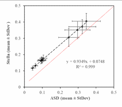
STELLA data was evaluated against measurements collected with an Analytical Spectral Devices spectrometer (ASD). An ASD is a common field instrument, calibrated to radiance, that provides stable reflectance estimates in the 400 – 2,500 nm region with a 3 nm spectral resolution. STELLA and ASD data were both collected in situ using a white panel target under consistent light and acquisition (sun-sensor-target) geometry conditions.
While the STELLA reflectance measurements were significantly higher than those collected using the ASD, the two datasets were strongly correlated under these conditions and no significant differences in uncertainty were observed (figure). Generally, the standard deviation of the data were found to vary between 8 – 18% while the standard errors were found in the range of 3 – 6%, with the VIS bands having lower uncertainties than those in the red-edge and NIR bands.
What do the STELLA spectrometers measure?
STELLA-Q2 – Light intensity (uW/cm2), in the visible and near infrared wavelengths (in nanometers): 410, 435, 460, 485, 510, 535, 560, 585, 610, 645, 680, 705, 730, 760, 810, 860, 900, 940
The light intensity is measured in microwatts per centimeters squared, with error bars of +/- 12% of the value. The sensor selects the specific wavelength bands by using a set of silicon thin-film interference filters, to a precision of +/- 5 nanometers. The bands are centered around the wavelengths listed above, and the bandwidth of each band is +/- 10 nanometers full-width half-maximum around the band center, in a Gaussian distribution of sensitivity. Silicon is a hard material with low thermal expansivity, so the sensor characteristics are stable over a broad temperature range, as well as over the life of the sensor. The sensor’s field of view is cone-shaped, with a cone angle of +/- 20° for a total field of view of 40°.
STELLA-Q, 1.0, 1.1 and 2.0 – Light intensity, in the visible wavelengths (in nanometers): 450, 500, 550, 570, 600, 650
The visible light intensity is measured in microwatts per centimeters squared, with error bars of +/- 12% of the value. The sensor selects the specific wavelength bands by using a set of silicon thin-film interference filters, to a precision of +/- 5 nanometers. The bands are centered around the wavelengths listed above, and the bandwidth of each band is +/- 20 nanometers full-width half-maximum around the band center, in a Gaussian distribution of sensitivity. Silicon is a hard material with low thermal expansivity, so the sensor characteristics are stable over a broad temperature range, as well as over the life of the sensor. The sensor’s field of view is cone-shaped, with a cone angle of +/- 20° for a total field of view of 40°.
STELLA-Q, 1.0, 1.1 and 2.0 – Light intensity (in microwatts per centimeters squared), in the near infrared wavelengths (in nanometers): 610, 680, 730, 760, 810, 860
The near infrared light intensity is measured in microwatts per centimeters squared, with error bars of +/- 12% of the value. The sensor selects the specific wavelength bands by using a set of silicon thin-film interference filters, to a precision of +/- 5 nanometers. The bands are centered around the wavelengths listed above, and the bandwidth of each band is +/- 10 nanometers full-width half-maximum around the band center, in a Gaussian distribution of sensitivity. Silicon is a hard material with low thermal expansivity, so the sensor characteristics are stable over a broad temperature range, as well as over the life of the sensor. The sensor’s field of view is cone-shaped, with a cone angle of +/- 20° for a total field of view of 40°.
STELLA-1.0, 1.1 and 2.0 – Surface temperature, in degrees Celsius. This sensor measures a far infrared light spectrum to produce a spectral curve. This curve is fit to a black-body thermal emission curve, to derive the surface temperature. This sensor is calibrated to objects that are emissive (not shiny metal surfaces). The temperature reading is good to +/- 0.5°C. The sensor’s field of view is cone-shaped, with a cone angle of +/- 17.5°, for a total field of view of 35°.
STELLA-1.0, 1.1 and 2.0 – Air temperature, in degrees Celsius. This sensor measures the ambient air temperature to an accuracy of +/- 0.25°C. It measures the semiconductor conduction-band quantum energy band-gap to derive the temperature. This method of measurement is accurate across a wide range of temperatures (-40 to +125°C) and is stable over the life of the sensor.
STELLA-1.0, 1.1 and 2.0 – Ambient conditions: Relative humidity, barometric pressure, altitude, and air temperature. This sensor measures those four parameters, though the air temperature measurement is less accurate than that of the MCP9808, so we do not record this sensor’s air temperature reading. The relative humidity measurement is good to +/- 3% and the barometric pressure reading, in hectoPascals, is good to +/-1 hPa. The altitude measurement is uncalibrated, so the absolute value is not accurate. The precision of the altitude measurement is better than 0.1%, so we include it to allow data marking by altitude excursion (a quick rise and fall) if the STELLA is in use on an aerial drone. In this way, the drone data and the STELLA data can be synchronized.
All STELLAs – Time. The clock on the STELLA is set to Coordinated Universal Time (UTC) to avoid confusion of time zones and daylight savings time. The clock is powered by the backup battery and will continue to keep time, even when the STELLA is off. The accuracy of this clock chip is +/- 2 seconds per day, about +/- 12 minutes per year.
Calibration Q & A
Jesse Barber, STELLA Calibration and Validation
How do we calibrate our sensors?
We calibrate our sensors radiometrically, which means that we use a broadband light source that is well defined as to how much power per unit wavelength per unit area is coming off of the source. Knowing how the source behaves, we can then look at our sensor and see how it’s data is different. We can then, after taking the measurement and gathering data, use a correction table to adjust the data coming off of the sensor to match what our source claims.
Why do we need calibration?
We calibrate our sensors for a few reasons,
1: We cant be sure exactly how the sensors react to stimuli out of the factory. Each batch of silicon will be slightly different, leading to sensors built from year to year possibly having a different signature. We calibrate against a known source to make sure that the sensors are within factory calibrations and error bounds. And even if they are not, we then create a new set of data so that we understand by how far off the stellas could be from each other and the true value. This set of error data can then inform those who do not have our calibration equipment how far off their data might be from the truth.
2: Sensors and technology changes and degrades over time. Calibration against a source that is very well understood over years can tell us how long stellas might last without any calibration. And how to adjust for the drift over the years.
What set up do you use?
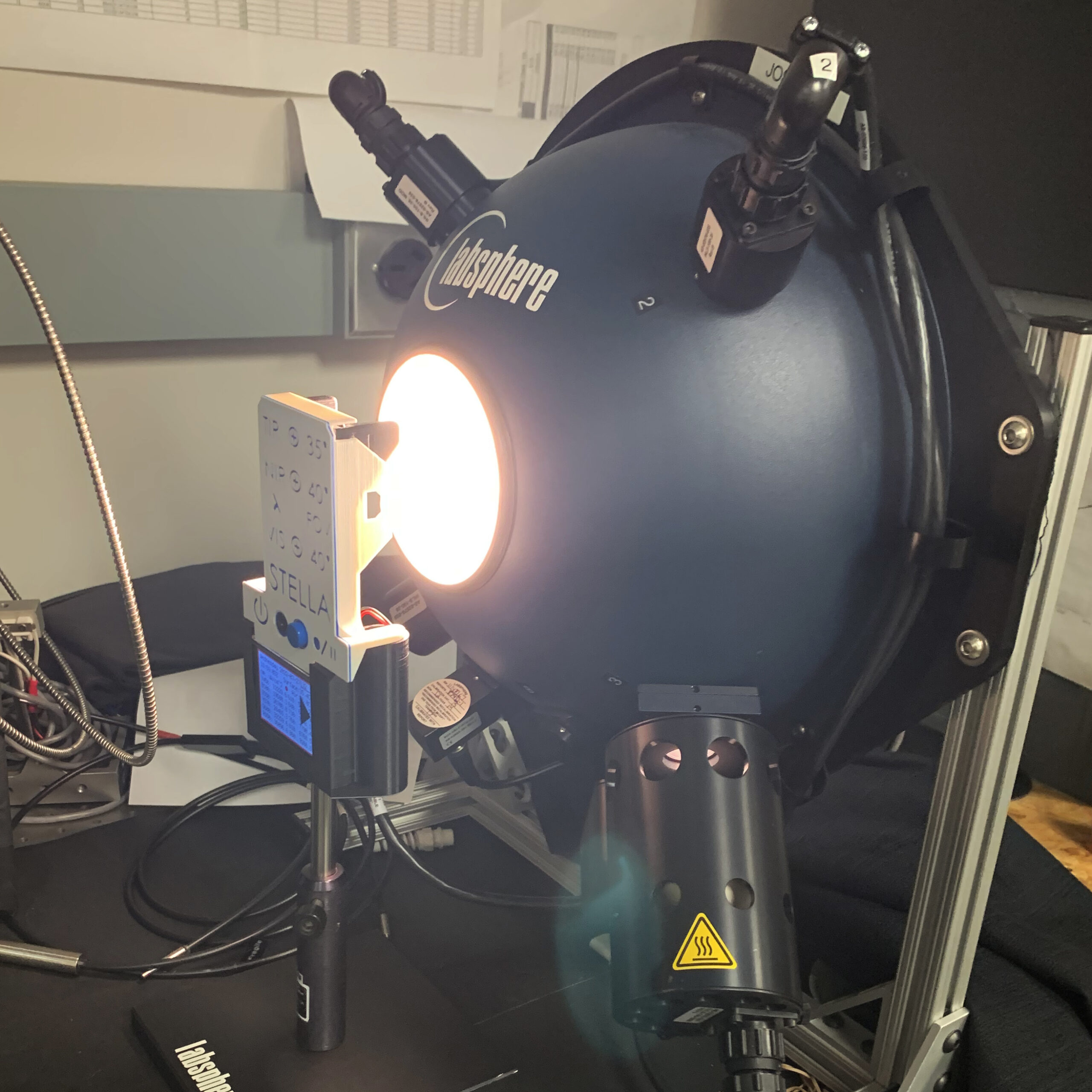
I use a LabSphere 12 in integrating sphere as my source. This produces a very even, diffuse circle of light 4” in diameter. In one calibration test, I turn on the lamps in my sphere and look directly into the light. This is the most accurate and repeatable calibration test.
In another I add a diffusely reflective matte white panel into the system, and have the light from my sphere reflect off of the panel and into the sensor. This angle of reflection is as small as possible without the sensor casting a shadow on the panel.
In the final calibration test I take my panel, and replace it with a piece of sanded, white foam board. My panel is a laboratory grade surface that is 99% reflective from 350nm to 2500 nm. The foam is from a craft store. We do this to attempt to allow for those customers/users to be able to calibrate a stella on their own at a low cost. And hopefully less than a 5-8% error compared to our lab grade equipment in the range that Stella operates.

What variables do we try and control for?
We try to control how much light gets into the sensors, at what angle it enters the sensors, the distance at which the sensor sits from the source, and the humidity in the air to name a few. All of these, not including humidity, will change the resulting reading systematically, effecting the calibration. Humidity only effects one band in the infrared, but it is still good to control for.
What variables can’t we control?
We cant control how each sensor comes from the factory, so any defects that get past quality control could change our data values by some percentage.
In most cases, this deviation is going to be within the factory’s calibration error bounds and will not effect most customers, but it is important to know when we have a deviation from the norm.
We also cant control how sensors will behave over time, and so we have to observe them and correct for them.

Why is it important to continue to check our calibration?
Sensor performance can degrade and change over time. So we calibrate at regular intervals with the same sensors to see how the sensors change and can inform our customers/users.
Julia Barsi, Landsat Radiometric Calibration Analyst GLAMR Science Manager
How do we calibrate our sensors?
In the laboratory, calibration is usually performed in a controlled environment with a known reference target that is very well understood. Targets for the visible and near-infrared regions of the spectrum include diffuser panels and integrating spheres that have known reflectances which are illuminated with lamps or lasers that have known emitted radiances. Targets for the thermal region of the spectrum are usually blackbodies which emit a very stable temperature. The reference targets are generally very flat, so the sensor sees nothing but a uniform field.
The sensor is looks at the target, which generates some electronic response. The response is recorded along with the property of the reference target. The ratio of the sensor response to the target property is the radiometric calibration of the sensor.
Why do we need calibration?
We need calibration to be able to make quantitative assessments of the physical properties being measured. The calibration allows us to convert the electronic signal (current or voltage?) in the STELLA instrument to the light intensity (microwatts per centimeter squared) or temperature (degrees Celsius). The calibration puts an absolute scale on the measurement that then can be quantitatively compared to other measurements.
Without calibration, we might be able to say that one plant is greener than another plant, for instance. But with calibration, we can say exactly how much greener one plant is and perhaps build a model of how greenness indicates plant health, for example.
What variables do we try and control for?
Calibration is usually performed in a controlled environment to ensure that the sensor is only responding the physical input under test and not outside influences. The internal temperature of the sensor may impact its responsiveness so it would be important to calibrate the sensor at the range of temperature conditions under which it would be used. The illumination conditions are generally controlled so that only light coming from the reference target is shining on the sensor.
Why is it important to continue to check our calibration?
Sensors can change over time. Sometimes a film builds up on mirrors or lenses making the optical path less transmissive. Sometimes the detector material degrades which causes loss of responsiveness. These changes can happen slowly or they can happen suddenly. And they will change the relationship between the sensor response and the physical parameter. If the calibration is not checked, the sensor response may have changed, but the result is that the physical property being measured appears to have changed.
For example, if the optical path has become 25% less transmissive, the sensor will be 25% less responsive. Let’s say you measured a target at the beginning of the month that has a light intensity of 4 uW/cm2 and you repeat the measurement at the end of the month but now is it only 3 uW/cm2. With calibration, you would have known that the target would look 25% dark, but without calibration, you think the plant is less healthly.