Hierarchical Image Segmentation - Glossary

National Aeronautics and Space Administration

Goddard Space Flight Center

Data Analysis

	The "3D NASA Logo" image is used as an image segmentation test image. This image is 200 x 200 pixels with a 3-element vector at each pixel representing the red, green, and blue spectral values. As a control to test the quality across the differenct segmentation approach, the target global dissimilarity criterion is 10. In the event that the different segmentation approaches can not reach the global criterion value of 10, they will get as close as possible while striving for a like quality across the approaches.
		Figure 1 Segmentation: Logical Predicate Threshold: 42.0 Regions: 313 Global dissimilarity value: 10.09 Observations: The segmentation results are often poor with the region boundaries inappropriately following along the image scan lines. Also, the computational efficiency of this region growing approach is very poor.
		Figure 2 Segmentation: Region Dissimilarity Threshold: 26.0 Regions: 203 Global dissimilarity value: 10.03 Observations: The segmentation result is much closer to the original image with a sharp decrease in scan line dependence. The computational load is much more efficient.
		Figure 3 Segmentation: BSMSE based Region Dissimilarity Threshold: 3200.0 Regions: 162 Global dissimilarity value: 9.99 Observations: The computational load is still efficient and the number of regions has decreased, however the reappearance of scan line dependance has returned.
		Figure 4 Segmentation: BMMSE based Region Dissimilarity Threshold: 1850.0 Regions: 151 Global dissimilarity value: 9.96 Observations: The computational load is still efficient, and again the number of regions has decreased while producing a spatial structure close to the original image, however the scan line dependance is still present but to a lesser degree.
		Figure 5 Segmentation: HSWO Regions: 36 Global dissimilarity value: 10.14 Observations: This method utilized an iterative approach such that it could produce a quality hierarchical boundary map with no scan line dependance and a sharp decline in the number of regions. However, it had an inefficient computing time of appproximately 30 minutes for a 200 x 200 pixel image, not very efficient
		Figure 6 Segmentation: RHSWO Regions: 39 Global dissimilarity value: 10.13 Observations: This recursive approach maintained the high quality of HSWO with a few more regions only at the cost of a far more efficient computing time less than minute.
		Figure 7 Segmentation: RHSWO w/ Processing Window Artifact Elimination Regions: 34 Global dissimilarity value: 10.26 Observations: Aside from this approaches primary function, window artifact elimination, a beneficial side effect is the reduction in the spread of the region clusters, thereby maintaining quality with lesser regions.
		Figure 8 Segmentation: RHSEG w/ spclust_wght=1.0 Regions: 13 Disjointed Regions: 425 Global dissimilarity value: 9.93 Observations: This extremely computational efficient approach, took less than 30 secs to a produce 13 region segmentation result with more detail than the previous approaches; it allows disjointed region merging. Nevertheless, depending upon the application, this could be too much detail when striving for a target global dissimilarity criterion.
		Figure 9 egmentation: RHSEG w/ spclust_wght=0.1 Regions: 14 Disjointed Regions: 594 Global dissimilarity value: 9.69 Observations: This approach is just as computational efficient with a small number of regions while maintaining high detail. However, the number of disjointed regions is far less than previously, thus, depending on the application, it could be to much detail when striving for a specific global dissimilarity criterion.

Segmentation Approach Vs. Number of Regions Produced
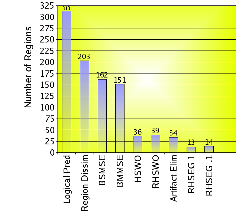	After obtaining close approximations of a global dissimilarity criterion value of 10 for each of the different approaches to image segmentation, this chart displays the difference in the number of regions produced from these approaches.
Region Growing Threshold vs Number of Regions Produced
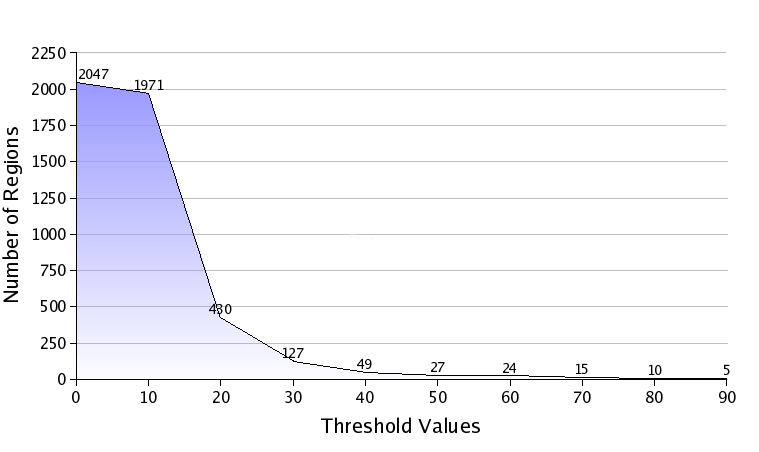	Chart 2 displays the relationship between the region growing threshold value and the number of regions produced, whereas the Logical Predicate Segmentation on "3D NASA Logo" is being used for the example. Although the Logical Predicate Segmentation results are displayed in the chart, the relationship between the threshold value and the number of regions holds true for all segmentation approaches: Logical Predicate Segmentation through BMMSE Region Dissimilarity Based, whose thresholds are iterated independently by the user, and HSWO through RHSEG, whose thresholds are iterated by the algorithm. From the information presented, it can be inferred that the region growing threshold value and the number of regions produced have an inverse relationship.
Region Growing Threshold vs. Global Dissimilarity Criterion Value Produced
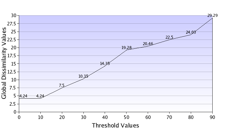	Chart 3 displays the relationship between the region growing threshold value and global dissimilarity criterion value produced, whereas the Logical Predicate Segmentation on "3D NASA Logo" is being used for the example. Although the Logical Predicate Segmentation results are displayed in the chart, the relationshiop between the threshold value and the global dissimilarity criterion values holds true for all segmentation approaches: Logical Predicate Segmentation through BMMSED Region Dissimilarity Based, whose thresholds are iterated independently by the user, and HSWO through RHSEG, whose thresholds are iterated by the algorithm. From the information presented, it can be inferred that the region growing threshold value and the global dissimilarity criterion value have a direct relationship.
Spectral Clustering produced Number of Regions vs. Global Dissimilarity Criterion Value Produced
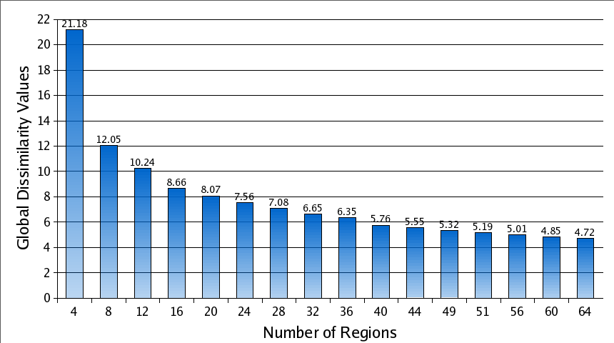	Chart 4 displays the relationship between the spectral clustering weight value and global dissimilarity criterion value produced on the premise that the independent variable is the number of regions. For this example, the spclust_wght is 1.0 as an addendum to the BSMSE Based Region Dissimilarity Function and the Processing Window Artifact Elimination algorithm activated. In this particular diagram, their is a inverse relationship between the number of regions and the global dissimilarity criterion value; meaning, that as the number of regions increase, the global dissimilarity criterion value decreases. Although, a spectral clustering weight of 1.0 is being used, the same relationship holds true for all spectral clustering weight between 1.0 and 0.1, however the values will vary based on the image.
Spectral Clustering Weight Value vs. Global Dissimilarity Value
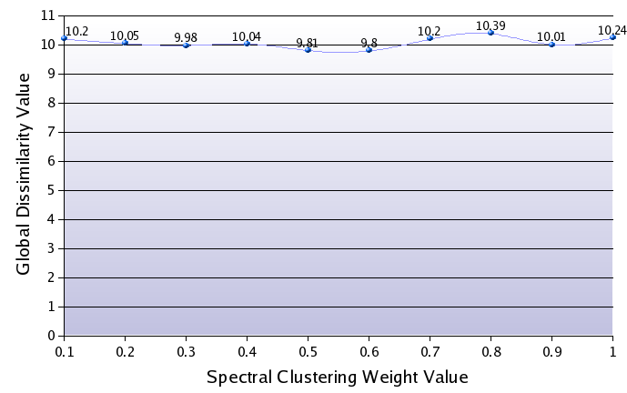	Chart 5 displays the relationship between the spectral clustering weight value and the global dissimilarity criterion value produced. The results displayed are produced by using the spectral clustering weight as the independent variable and a region number of 12 for the control. This chart utilizes results from processing the "3D NASA Logo" with the BSMSE based Region Dissimilarity Function and Processing Window Artifact Elimination algorithm. An analysis of the results show that a definite relationship does not exist. Although not pictured, other images' results using the same comparison and algorithm displayed a wavy, unstable movement, but not identical to the pattern of hills and valleys like Chart 5. Thus, it can be inferred that the specral clustering weight produces varied global dissimilarity criterion values as it is strictly dependent upon the image spectral attributes.