Research Page
Geomagnetism
Geomagnetism: modeling and separation of Earth's magnetic field sources to enable a better understanding of the underlying generating mechanisms
Terence J. Sabaka (Code 61A, NASA GSFC)
Robert H. Tyler (University of Maryland @ Code 61A, NASA GSFC)
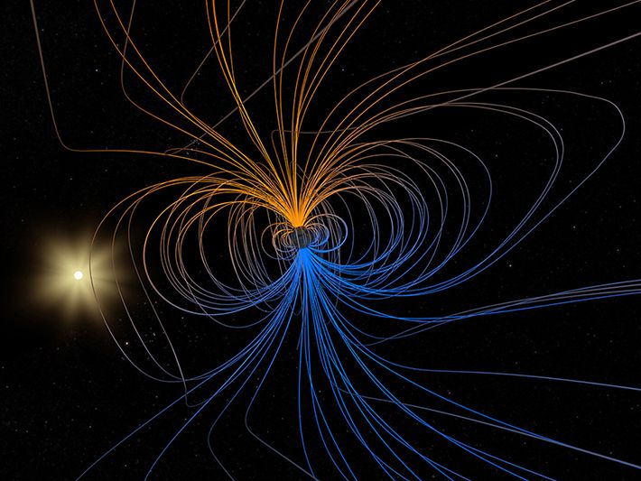
A single measurement of the near-Earth magnetic field (within 1500 km of the surface) is comprised of a superposition of signals from different current sources within the system. In order to study a particular source, it must be separated from the others using inverse theory in which the geophysical parameters of a model are inferred from field measurements. These measurements are most often provided by magnetometer measurements on board satellites and from permanent ground-based stations.
To this end, the NASA/GSFC magnetism group, along with the Danish Technical Institute, has developed an approach called "Comprehensive Modeling" (CM), which parameterizes most major near-Earth sources and subsequently co-estimates them in order to achieve optimal source separation. These sources include the core, lithosphere, M2 tidal, magnetosphere, ionosphere, associated induced fields, and toroidal fields inside satellite sampling shells. This co-estimation is key to the great success of the CMs and can be understood by the Venn diagram in Figure 1, which shows a data space D and two parameter spaces A and B. In most cases A and B have a non-empty intersection, "A intersection B", which causes non-uniqueness when sequential estimation is used. However, co-estimation eliminates this region and extracts the parameters of A and B from "A minus B" and "B minus A", respectively, for optimal separation.
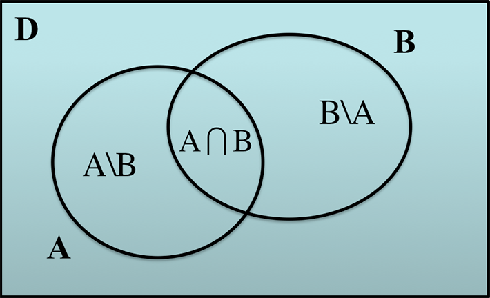
Figure 1: Venn Diagram depicting the relationship between a data space and the span of two model parameter spaces.
The error between the true and model parameter values consists of bias and variance. While most models only consider variance, the CMs also consider bias. This is shown in Figure 2, where the total error (blue lines) is decomposed into variance about an ensemble mean (dotted red lines) and the bias between the ensemble mean and truth (solid red line). The accounting for bias allows the CMs to co-estimate sources from heterogeneous data sets that are sensitive (high signal-to-noise rations) to only a sub-set of parameters.
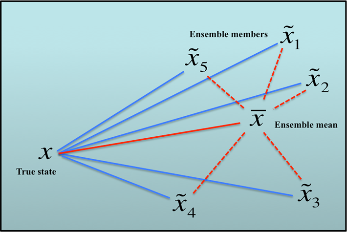
Figure 2: Error between true and model states can be decomposed into variance and bias portions.
Theoretical study and forward numerical simulation of geophysical electrodynamic processes are important in the continuing development of the parametric bases of the CM model, and in validating results. The NASA/GSFC magnetism group develops numerical models for simulating the magnetic (and electric) fields associated with induction and motional induction sources near the Earth's surface and oceans. This development includes more general 3D approaches (Tyler et al., 2004) but focus is currently on sources with very large scales, and periods much longer than about ten minutes. For this purpose, a Thin-Shell Induction Model (TSIM) has been developed that allows fast, high-resolution, global simulations where the realistic ocean is inductively coupled to a mantle with radially dependent electrical conductivity (Tyler et al., 2003; Sabaka et al., 2015, 2016; Tyler 2017).
As a testament to the effectiveness of combining the CM approach with TSIM validation, the magnetic signal from the M2 semi-diurnal lunar tide has been extracted from CHAMP satellite data in the CM5 model (Sabaka et al., 2015), one of a suite of CMs produced, and is shown in the bottom panel of Figure 3.
The middle panel of Figure 3 shows the M2 tidal magnetic signal as predicted by TSIM. This simulation uses as input the OSU TPX8.1 tidal flow (Egbert, G.D., and S.Y. Erofeeva, 2002 ), and the recently compiled climatology data base of ocean electrical conductivity (Tyler et al., 2017) shown in Figure 4.
The agreement with these two independent results provides strong validation that CM has indeed extracted the realistic M2 signal due to ocean tides (as opposed to atmospheric tides, for example). It also provides validation of the TSIM modeling approach and allows confidence in the predictions of additional TSIM source signals that become a goal in the resolution of further CM development.
Figure 3: A movie of the sea surface displacement due to the lunar semi-diurnal (M2) tide is shown in the top panel. The middle panel shows the radial component of the surface magnetic field as predicted by TSIM. The bottom panel shows the M2 signal extracted by CM from observations. The agreement in the independently derived theoretical and observed M2 signals provides strong cross validation. Disagreement is mostly due to the higher spatial resolution currently included in the prediction.
Figure 4: The distribution of annual mean electrical conductivity (S/m) of the 3-D, global ocean is shown as movie frames for depths ranging from the surface to the sea floor.
For more information, please contact Terry Sabaka or Rob Tyler
References
Egbert, G.D., and S.Y. Erofeeva (2002). Efficient inverse modeling of barotropic ocean tides, J. Atmos. Oceanic Technol., 19, 2, p.183-204. doi: 10.1175/1520-0426(2002)019<0183:EIMOBO>2.0.CO;2
Sabaka, T.J., Tyler, R.H., and N. Olsen (2016). Extracting ocean-generated tidal magnetic signals from Swarm data through satellite gradiometry, Geophys. Res. Lett., 43, doi:10.1002/2016GL068180.
Sabaka, T.J., Olsen, N., Tyler, R.H., and A. Kuvshinov (2015). CM5, a pre-Swarm comprehensive geomagnetic field model derived from over 12 yr of CHAMP, Oersted, SAC-C and observatory data, Geophys. J. Intl., 200, 1596-1626, doi:10.1093/gji/ggu493.
Sabaka, T.J., Toffner-Clausen, L., and N. Olsen (2013). Use of the comprehensive inversion method for Swarm satellite data analysis, Earth, Planets and Space, 65, 1202-1222,doi:10.5047/eps.2013.09.007
Sabaka, T.J., and N. Olsen (2006). Enhancing comprehensive inversions using the Swarm constellation, Earth, Planets and Space, 58, 371-395, doi:10.1186/BF03351935.
Sabaka, T.J., Olsen, N., and M.E. Purucker (2004). Extending comprehensive models of the Earth's magnetic field with Oersted and CHAMP data, Geophys. J. Int., 159, 521-54, doi:10.1111/j.1365-246X.2004.02421.x.
Sabaka, T.J., Olsen, N., and R.A. Langel (2002). A comprehensive model of the quiet-time near-Earth magnetic field: phase 3, Geophys. J. Intl., 151, 32-68, doi:10.1046/j.1365-246X.2002.01774.x
Tyler, R. H. (2017). Mathematical Modeling of Electrodynamics near the surface of Earth and Planetary Water Worlds. NASA TM-2017-219022.
Tyler, R. H., Boyer, T. P., Minami, T., Zweng, M. M. & Reagan, J. R. (2017). Electrical conductivity of the global ocean, Earth, Planets and Space, 69, 156 (2017), doi: 10.1186/s40623-017-0739-7.
Tyler, R. H., Maus, S. and Lühr, H. Satellite Observations of Magnetic Fields Due to Ocean Tidal Flow (2003). Science, 299, 239-241. doi: 10.1126/science.1078074.
Tyler, R. H., Vivier, F. & Li, S. (2004). Three-dimensional modelling of ocean electrodynamics using gauged potentials. Geophysical Journal International 158, 874-887. doi: 10.1111/j.1365-246X.2004.02318.x.
Terence J. Sabaka (Code 61A, NASA GSFC)
Robert H. Tyler (University of Maryland @ Code 61A, NASA GSFC)
A single measurement of the near-Earth magnetic field (within 1500 km of the surface) is comprised of a superposition of signals from different current sources within the system. In order to study a particular source, it must be separated from the others using inverse theory in which the geophysical parameters of a model are inferred from field measurements. These measurements are most often provided by magnetometer measurements on board satellites and from permanent ground-based stations.
To this end, the NASA/GSFC magnetism group, along with the Danish Technical Institute, has developed an approach called "Comprehensive Modeling" (CM), which parameterizes most major near-Earth sources and subsequently co-estimates them in order to achieve optimal source separation. These sources include the core, lithosphere, M2 tidal, magnetosphere, ionosphere, associated induced fields, and toroidal fields inside satellite sampling shells. This co-estimation is key to the great success of the CMs and can be understood by the Venn diagram in Figure 1, which shows a data space D and two parameter spaces A and B. In most cases A and B have a non-empty intersection, "A intersection B", which causes non-uniqueness when sequential estimation is used. However, co-estimation eliminates this region and extracts the parameters of A and B from "A minus B" and "B minus A", respectively, for optimal separation.
Figure 1: Venn Diagram depicting the relationship between a data space and the span of two model parameter spaces.
The error between the true and model parameter values consists of bias and variance. While most models only consider variance, the CMs also consider bias. This is shown in Figure 2, where the total error (blue lines) is decomposed into variance about an ensemble mean (dotted red lines) and the bias between the ensemble mean and truth (solid red line). The accounting for bias allows the CMs to co-estimate sources from heterogeneous data sets that are sensitive (high signal-to-noise rations) to only a sub-set of parameters.
Figure 2: Error between true and model states can be decomposed into variance and bias portions.
Theoretical study and forward numerical simulation of geophysical electrodynamic processes are important in the continuing development of the parametric bases of the CM model, and in validating results. The NASA/GSFC magnetism group develops numerical models for simulating the magnetic (and electric) fields associated with induction and motional induction sources near the Earth's surface and oceans. This development includes more general 3D approaches (Tyler et al., 2004) but focus is currently on sources with very large scales, and periods much longer than about ten minutes. For this purpose, a Thin-Shell Induction Model (TSIM) has been developed that allows fast, high-resolution, global simulations where the realistic ocean is inductively coupled to a mantle with radially dependent electrical conductivity (Tyler et al., 2003; Sabaka et al., 2015, 2016; Tyler 2017).
As a testament to the effectiveness of combining the CM approach with TSIM validation, the magnetic signal from the M2 semi-diurnal lunar tide has been extracted from CHAMP satellite data in the CM5 model (Sabaka et al., 2015), one of a suite of CMs produced, and is shown in the bottom panel of Figure 3.
The middle panel of Figure 3 shows the M2 tidal magnetic signal as predicted by TSIM. This simulation uses as input the OSU TPX8.1 tidal flow (Egbert, G.D., and S.Y. Erofeeva, 2002 ), and the recently compiled climatology data base of ocean electrical conductivity (Tyler et al., 2017) shown in Figure 4.
The agreement with these two independent results provides strong validation that CM has indeed extracted the realistic M2 signal due to ocean tides (as opposed to atmospheric tides, for example). It also provides validation of the TSIM modeling approach and allows confidence in the predictions of additional TSIM source signals that become a goal in the resolution of further CM development.
Figure 3: A movie of the sea surface displacement due to the lunar semi-diurnal (M2) tide is shown in the top panel. The middle panel shows the radial component of the surface magnetic field as predicted by TSIM. The bottom panel shows the M2 signal extracted by CM from observations. The agreement in the independently derived theoretical and observed M2 signals provides strong cross validation. Disagreement is mostly due to the higher spatial resolution currently included in the prediction.
Figure 4: The distribution of annual mean electrical conductivity (S/m) of the 3-D, global ocean is shown as movie frames for depths ranging from the surface to the sea floor.
For more information, please contact Terry Sabaka or Rob Tyler
References
Egbert, G.D., and S.Y. Erofeeva (2002). Efficient inverse modeling of barotropic ocean tides, J. Atmos. Oceanic Technol., 19, 2, p.183-204. doi: 10.1175/1520-0426(2002)019<0183:EIMOBO>2.0.CO;2
Sabaka, T.J., Tyler, R.H., and N. Olsen (2016). Extracting ocean-generated tidal magnetic signals from Swarm data through satellite gradiometry, Geophys. Res. Lett., 43, doi:10.1002/2016GL068180.
Sabaka, T.J., Olsen, N., Tyler, R.H., and A. Kuvshinov (2015). CM5, a pre-Swarm comprehensive geomagnetic field model derived from over 12 yr of CHAMP, Oersted, SAC-C and observatory data, Geophys. J. Intl., 200, 1596-1626, doi:10.1093/gji/ggu493.
Sabaka, T.J., Toffner-Clausen, L., and N. Olsen (2013). Use of the comprehensive inversion method for Swarm satellite data analysis, Earth, Planets and Space, 65, 1202-1222,doi:10.5047/eps.2013.09.007
Sabaka, T.J., and N. Olsen (2006). Enhancing comprehensive inversions using the Swarm constellation, Earth, Planets and Space, 58, 371-395, doi:10.1186/BF03351935.
Sabaka, T.J., Olsen, N., and M.E. Purucker (2004). Extending comprehensive models of the Earth's magnetic field with Oersted and CHAMP data, Geophys. J. Int., 159, 521-54, doi:10.1111/j.1365-246X.2004.02421.x.
Sabaka, T.J., Olsen, N., and R.A. Langel (2002). A comprehensive model of the quiet-time near-Earth magnetic field: phase 3, Geophys. J. Intl., 151, 32-68, doi:10.1046/j.1365-246X.2002.01774.x
Tyler, R. H. (2017). Mathematical Modeling of Electrodynamics near the surface of Earth and Planetary Water Worlds. NASA TM-2017-219022.
Tyler, R. H., Boyer, T. P., Minami, T., Zweng, M. M. & Reagan, J. R. (2017). Electrical conductivity of the global ocean, Earth, Planets and Space, 69, 156 (2017), doi: 10.1186/s40623-017-0739-7.
Tyler, R. H., Maus, S. and Lühr, H. Satellite Observations of Magnetic Fields Due to Ocean Tidal Flow (2003). Science, 299, 239-241. doi: 10.1126/science.1078074.
Tyler, R. H., Vivier, F. & Li, S. (2004). Three-dimensional modelling of ocean electrodynamics using gauged potentials. Geophysical Journal International 158, 874-887. doi: 10.1111/j.1365-246X.2004.02318.x.